Is Trend Your Friend?
Understanding Trend, Support, and Resistance — A Simple Guide Before the Code
When you start exploring the financial markets, three core concepts come up over and over again: trend, support, and resistance. While they might sound technical, they’re simply ways to understand how prices move — and where they often pause, reverse, or break through.
Let’s walk through them in plain terms.
What Is a Trend?
A trend is the general direction in which a market is moving.
-
If prices are steadily rising, it’s called an uptrend.
-
If prices are generally falling, it’s a downtrend.
-
If prices are moving sideways without much direction, that’s called consolidation or a sideways trend.
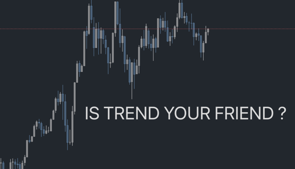
There’s a popular saying in trading: “The trend is your friend.” That’s because traders often look to follow the trend rather than go against it — much like riding the current instead of swimming upstream.
What Is Support?
Support is a price level where a falling market tends to pause, attract buying interest, and potentially bounce back up. Think of it as a floor beneath the price — a level where downward momentum often slows or reverses.
Support forms when traders believe the price has dropped low enough to become attractive again. As buyers step in, their demand helps push the price back up.
An important behavior to understand:
If the price breaks below a support level, it often comes back to retest that level from underneath before continuing lower. In this case, the old support can turn into new resistance.
Also, if the overall trend is strong, the price may eventually return to the trend zone — the broader area where the uptrend or downtrend has been developing — even after briefly breaking below support. This means support is not always a strict line but can be part of a larger structure where price fluctuates before resuming the dominant trend.
What Is Resistance?
Resistance is a price level where a rising market tends to stall, attract selling pressure, and potentially reverse downward. You can think of it as a ceiling — a level where upward momentum often slows or turns back.
Resistance forms when traders believe the price has risen high enough to start selling. As more sellers enter the market, the increased supply can push the price down.
An important behavior to understand:
If the price breaks above a resistance level, it often comes back to retest that level from above before moving higher. In this case, the old resistance can become new support.
Also, if the underlying trend is strong, the price may eventually return to the trend zone — the general upward path it was following — even after temporarily pulling back from or above resistance. This highlights how resistance isn’t always a fixed ceiling, but part of a larger price structure within a trend.
Why Support and Resistance Matter
Support and resistance help traders identify key decision zones:
-
Buying near support can offer good risk-reward setups.
-
Selling near resistance allows traders to take profits before a potential pullback.
-
Watching how price reacts to these levels can help determine whether a trend will continue or reverse.
These levels are also key areas to watch for breakouts and retests, which often lead to stronger price movements.
Combining Trend with Support and Resistance
The real advantage comes when you combine trend direction with support and resistance:
-
In an uptrend, traders often buy on pullbacks near support.
-
In a downtrend, traders may sell on rallies near resistance.
This approach adds structure to your strategy. Instead of guessing, you’re working with a framework that reflects how markets naturally behave.
Putting It All Together
Now that you understand the core concepts, it’s time to see them in action.
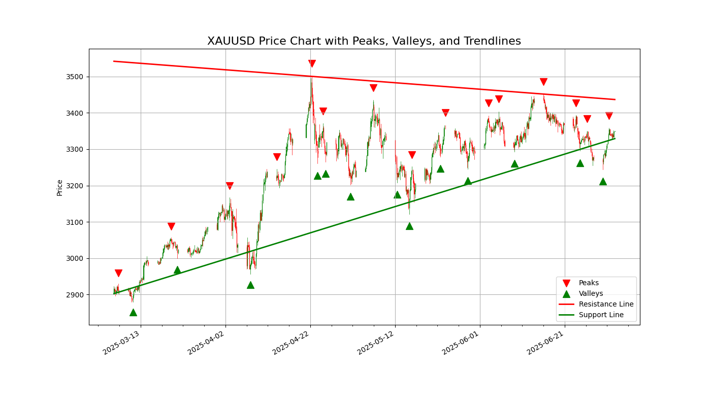
Below, you’ll find a Python script that fetches real market data and automatically draws support and resistance trend lines. This visual representation will help you recognize these patterns more clearly and strengthen your trading decisions.
Let’s move on to the code.
    from tvDatafeed import TvDatafeed, Interval
import pandas as pd
import numpy as np
import matplotlib.pyplot as plt
from matplotlib.dates import date2num, DateFormatter
from matplotlib.ticker import AutoMinorLocator
from mplfinance.original_flavor import candlestick_ohlc
from scipy.signal import argrelextrema
from datetime import datetime
from itertools import combinations

# Initialize TVDataFeed
tv = TvDatafeed()

# Parameters
ticker = 'XAUUSD'
exchange = 'OANDA'
start_date = datetime(2024, 1, 1)
end_date = datetime.now()

# Fetch historical data
data = tv.get_hist(
    symbol=ticker,
    exchange=exchange,
    interval=Interval.in_4_hour,
    n_bars=500,
    extended_session=False
)

# Prepare DataFrame
data.index = pd.to_datetime(data.index)
data = data.rename(columns={
    'open': 'Open', 'high': 'High',
    'low': 'Low', 'close': 'Close',
    'volume': 'Volume'
})
data = data[(data.index >= start_date) & (data.index <= end_date)]

# Convert to OHLC for candlestick_ohlc
data_ohlc = data[['Open', 'High', 'Low', 'Close']].copy()
data_ohlc['DateNum'] = date2num(data.index.to_pydatetime())
data_ohlc = data_ohlc[['DateNum', 'Open', 'High', 'Low', 'Close']]

# Find Peaks and Valleys
n = 10
high_idx = argrelextrema(data['High'].values, np.greater_equal, order=n)[0]
low_idx = argrelextrema(data['Low'].values, np.less_equal, order=n)[0]

def find_trendline_points_with_lowest(points_df, full_dates, lowest_pos,
                                      min_early=2, min_late=1, early_frac=0.2, late_frac=0.2):
    n_points = len(points_df)
    dates = points_df.index
    total_days = (full_dates[-1] - full_dates[0]).days
    early_cutoff = full_dates[0] + pd.Timedelta(days=int(total_days * early_frac))
    late_cutoff = full_dates[-1] - pd.Timedelta(days=int(total_days * late_frac))

    included = {lowest_pos}

    early_indices = [i for i, d in enumerate(dates) if d <= early_cutoff and i != lowest_pos]
    late_indices = [i for i, d in enumerate(dates) if d >= late_cutoff and i != lowest_pos]

    others = [i for i in range(n_points) if i != lowest_pos]

    for comb in combinations(others, 2):
        combined = set(comb) | included
        early_count = len([i for i in combined if i in early_indices])
        late_count = len([i for i in combined if i in late_indices])
        if dates[lowest_pos] <= early_cutoff:
            early_count += 1
        if dates[lowest_pos] >= late_cutoff:
            late_count += 1
        if early_count >= min_early and late_count >= min_late:
            return list(combined)
    return None

# Resistance line (2 highest peaks)
resistance_line = None
if len(high_idx) >= 2:
    recent_peaks = data.iloc[high_idx].nlargest(2, 'High')
    x_peak = date2num(recent_peaks.index.to_pydatetime())
    y_peak = recent_peaks['High'].values
    coeffs_res = np.polyfit(x_peak, y_peak, 1)
    resistance_line = np.poly1d(coeffs_res)

# Support line (valleys)
support_line = None
if len(low_idx) >= 3:
    valleys = data.iloc[low_idx]
    lowest_low_val = valleys['Low'].min()
    lowest_low_dt = valleys[valleys['Low'] == lowest_low_val].index[0]
    lowest_pos = list(valleys.index).index(lowest_low_dt)

    chosen_idx = find_trendline_points_with_lowest(valleys, data.index, lowest_pos)

    if chosen_idx is not None:
        selected_points = valleys.iloc[chosen_idx]
        x_vals = date2num(selected_points.index.to_pydatetime())
        y_vals = selected_points['Low'].values
        coeffs_sup = np.polyfit(x_vals, y_vals, 1)
        support_line = np.poly1d(coeffs_sup)

# Plotting
fig, ax = plt.subplots(figsize=(14, 8))

candlestick_ohlc(ax, data_ohlc.values, width=0.03, colorup='green', colordown='red', alpha=0.8)

# Peaks and Valleys
ax.scatter(date2num(data.iloc[high_idx].index.to_pydatetime()),
           data.iloc[high_idx]['High'] * 1.01,
           marker='v', color='red', s=100, label='Peaks')

ax.scatter(date2num(data.iloc[low_idx].index.to_pydatetime()),
           data.iloc[low_idx]['Low'] * 0.99,
           marker='^', color='green', s=100, label='Valleys')

# Resistance line
if resistance_line is not None:
    y_res = resistance_line(data_ohlc['DateNum'].values)
    ax.plot(data_ohlc['DateNum'].values, y_res, color='red', linewidth=2, label='Resistance Line')

# Support line
if support_line is not None:
    y_sup = support_line(data_ohlc['DateNum'].values)
    ax.plot(data_ohlc['DateNum'].values, y_sup, color='green', linewidth=2, label='Support Line')

# Format
ax.xaxis.set_major_formatter(DateFormatter('%Y-%m-%d'))
ax.xaxis.set_minor_locator(AutoMinorLocator())
fig.autofmt_xdate()

ax.set_title(f"{ticker} Price Chart with Peaks, Valleys, and Trendlines", fontsize=16)
ax.set_ylabel("Price")
ax.legend()
ax.grid(True)

plt.show()


